Differences between pythonradex and RADEX

Overlapping lines and internal continuum

pythonradex is able to handle excitation effects of overlapping lines (i.e. lines that are so close in frequency that photons emitted from one line can be absorbed by another line). pythonradex is also able to include effects of an internal radiation field specified by the user (typically arising from dust that is mixed with the gas). Both of these effects are not included in RADEX.

Programming language and performance

While RADEX is written in Fortran, pythonradex is written in python. Simple performance tests suggest that pythonradex outperforms RADEX in the typical use case of calculating several models over a grid of parameters (e.g. column density, temperature). The speed advantage of pythonradex from these tests ranges from ~2 up to more than 10, depending on the input parameters and the computing environment. To optimize its performance, pythonradex employs an architecture that avoids unnecessary or repeating calculations as much as possible. In addition, it uses just-in-time compilation using the numba package.

Different flux output

There is a difference between the outputs of RADEX and pythonradex. The RADEX output \(T_R\) (or the corresponding flux outputs) is intended to be directly compared to telescope data. To be more specific, from the optical depth and excitation temperature, RADEX first computes \(I_\mathrm{tot} = B_\nu(T_\mathrm{ex})(1-e^{-\tau}) + I_\mathrm{bg}e^{-\tau}\), i.e. the total specific intensity at the line centre that is recorded at the telescope, where \(I_\mathrm{bg}\) is the background radiation. This is the sum of the radiation from the gas (first term) and the background radiation attenuated by the gas (second term). From this, RADEX assumes the observer has subtracted the background, giving \(I_\mathrm{measured} = I_\mathrm{tot} - I_\mathrm{bg} = (B_\nu(T_\mathrm{ex})-I_\mathrm{bg})(1-e^{-\tau})\). The RADEX output \(T_R\) is the Rayleigh-Jeans temperature corresponding to \(I_\mathrm{measured}\). This output may or may not be the right quantity to be compared to observations. For example, it is almost certainly not appropriate to be compared to interferometric data. On the other hand, pythonradex outputs the pure line emission without any background subtraction, i.e. the output corresponds simply to the emission emitted by the gas (for a slab geometry, the fluxes would be based on the specific intensity given simply by \(B_\nu(T_\mathrm{ex})(1-e^{-\tau}))\). This allows the user to decide how the flux should be compared to observations.

Different specific intensity and flux for spherical geometry

For a given excitation temperature \(T_{ex}\) and optical depth \(\tau\), RADEX calculates the specific intensity as

\[I_\nu = B_\nu(T_{ex})(1-e^{-\tau})\]

for all geometries. However, this expression is only valid for slab geometries, but not for spherical geometries (“static sphere” and “LVG sphere”). In contrast, pythonradex uses different formulae for spherical geometries (see the section about geometries for more details).

For a static sphere, the specific intensity depends on the position on the sphere: if one looks towards the center of the sphere, it will be brighter than the sphere edges (because when looking through the center, the column density is higher), unless the sphere is completely optically thick. Therefore, the specific intensity, or brightness temperature, computed by RADEX using the above equation corresponds to what one would observe towards the center of the sphere if the observations resolved the sphere. On the other hand, pythonradex computes a sort of mean specific intensity, in the sense that if that specific intensity is multiplied by the solid angle of the sphere (\(R^2\pi/d^2\), with \(R\) the physical radius of the sphere and \(d\) the distance), you get the correct total flux density. So the specific intensity computed by pythonradex corresponds to what one would measure from completely unresolved observations (assuming an appropriate beam-filling factor is applied).

Similarly, for an LVG sphere, RADEX returns the specific intensity towards the center of the sphere, while pythonradex returns a specific intensity such that if multiplied by the solid angle, the correct flux density is computed. In addition, pythonradex computes the correct frequency dependence of the specific intensity (see Source geometries).

Whether resolved or unresolved, pythonradex gives the correct total flux (W/m²) emitted by the whole sphere, while RADEX might not (depending on the optical depth and geometry). The following figure illustrates the difference in flux that results from using different formulae. For a static sphere, using the slab formula (as done by RADEX) overestimates the flux in the optically thin limit by a factor 1.5. This factor simply represents the volume ratio between a “spherical slab” (i.e. a cylinder) and a sphere. In the optically thick limit, only the surface of the static sphere is visible, so either formula gives the same result. On the other hand, for the LVG sphere, the difference is always a factor 1.5, regardless of optical depth. This is due to the LVG assumption that all photons escape unless absorbed locally.

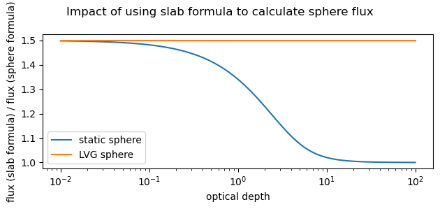
For the two spherical geometries, we computed the flux using the slab formula (as done by RADEX) and formulae appropriate for a sphere (as done by pythonradex). The figure shows the ratio of the fluxes as function of optical depth.

To verify that pythonradex calculates the flux correctly, one may consider the optically thin limit where the flux can be calculated directly. In this limit, all photons escape the source. The total flux (in [W/m²]) is then simply given by

\[F_\mathrm{thin} = V_\mathrm{sphere}nx_2A_{21}\Delta E \frac{1}{4\pi d^2}\]

where \(V_\mathrm{sphere}=\frac{4}{3}R^3\pi\) is the volume of the sphere, \(n\) the constant number density, \(x_2\) the fractional level population of the upper level, \(A_{21}\) the Einstein coefficient, \(\Delta E\) the energy difference between the upper and lower level, and \(d\) the distance of the source. pythonradex correctly reproduces this limiting case, but RADEX overestimates the optically thin flux by a factor 1.5.

Flux calculation

RADEX computes the flux by assuming that the flux density has a Gaussian profile (see Appendix A.2, point 5, in [vanderTak07]). However, for optically thick lines, the flux density profile is not Gaussian, even if the intrinsic line profile (and thus optical depth profile) is. On the other hand, pythonradex calculates the flux by integrating over the flux density profile, thus taking its shape into account. Note though, as commented by [vanderTak07], that proper modelling of optically thick lines cannot really be achieved anyway by 1D codes like RADEX or pythonradex.

Different escape probability for LVG sphere

For the spherical LVG geometry, RADEX and pythonradex use different formulae to calculate the escape probability. Please see the section about geometries for more details.

Different behaviour for H₂ collider densities

Whenever the LAMDA-formatted molecular data file contains collisional rates for H₂, but the user does not provide an H₂ density, RADEX just adds an H₂ density of \(10^5\) cm^-3 by default to the calculation.

Furthermore, if the molecular data file contains rates for ortho-H₂ and para-H₂, but not for H₂, and the user supplies an H₂ density instead of densities for ortho-H₂ and para-H₂, then RADEX will convert the supplied H₂ density into densities of H₂ and H₂ assuming a thermal ortho/para ratio.

On the other hand, pythonradex does not add H₂ by default, nor allow the user to request colliders that are not present in the molecular data file.