Getting started with pythonradex

pythonradex is used to solve the non-LTE radiative transfer in a 1D geometry. It can include effects of dust continuum and overlapping lines. Here we look at the main functionalities provided by pythonradex.

Note that all input and output for pythonradex is in SI units.

Initialisation

In pythonradex, a radiative transfer calculation is conducted using the Source class which is provided by the radiative_transfer module. Let’s have a look how to initialise it. Please refer to the API for more details

from pythonradex import radiative_transfer, helpers
from scipy import constants
import numpy as np
import matplotlib.pyplot as plt

First we need to initialise an instance of the Source class. The input parameters are as follows:

• datafilepath: Filepath to the file containing molecular data. The file needs to follow the LAMDA format and is usually downloaded from the EMAA database or the LAMDA database.

• geometry: The geometry of the source. Please see the documentation for more details about the geometries. Available options: ‘static sphere’, ‘static slab’, ‘LVG slab’, ‘LVG sphere’, ‘static sphere RADEX’ (emulating RADEX), ‘LVG sphere RADEX’ (emulating RADEX).

• line_profile_type: The shape of the intrinsic emission line profile. Available options: ‘rectangular’ and ‘Gaussian’. Note that for LVG geometries, only rectangular is allowed.

• width_v: The width of the emission line in velocity space. For a Gaussian, this corresponds to the FWHM. Note that pythonradex uses SI units, so this needs to be given in m/s.

• use_Ng_acceleration: Whether to use Ng acceleration to speed up convergence. Defaults to True.

• treat_line_overlap: Whether to treat line overlap effects (i.e. emission lines that overlap in frequency). This option is computationally expensive. Not allowed for LVG geometries. Defaults to False. There is a dedicated example notebook demonstrating this capability.

• warn_negative_tau: Whether to throw a warning in the case where negative optical depth occurs for any transition. Defaults to True.

• verbose: Whether to print out additional info. Defaults to False.

• test_mode: Whether to activate test mode. Only for developers, should be left to its default, i.e. False.

Let’s initialise a source. In this example, we consider CO. We leave some parameters at their default values.

datafilepath = "./co.dat"  # CO
geometry = "static sphere"
line_profile_type = "Gaussian"
width_v = 1.5 * constants.kilo  # 1500 m/s = 1.5 km/s

source = radiative_transfer.Source(
    datafilepath=datafilepath,
    geometry=geometry,
    line_profile_type=line_profile_type,
    width_v=width_v,
)

Setting the source parameters

Next, we are going to set the parameters characterising the source physical conditions. These parameters are:

• N: The column density, in units of m\(^{-2}\). For spherical geometries, this is the column density along the diameter of the sphere.

• Tkin: The kinetic temperature of the gas in units of K.

• collider_densities: The number density of colliders, in dictionary format, in units of m\(^{-3}\). The following colliders are recognised: “H2”, “para-H2”, “ortho-H2”, “e”, “H”, “He”, “H+”. Obviously, only colliders present in the data file can be used here.

• ext_background: The external background radiation. This is the radiation field that irradiates the source from the exterior and can affect the excitation conditions. The user can provide a custom radiation field by providing a function that takes a frequency array as input and returns the radiation field in units of W/m\(^2\)/Hz/sr. The commonly used CMB background can by used via the helpers module. One can also set this parameter to a number, which is interpreted as a constant value for all frequencies. So if no external background is desired, simply set this parameter to 0. Examples: ext_background = lambda nu: helpers.B_nu(nu=nu,T=200) (a black body at 200 K); ext_background = 0 (no external background); ext_background = helpers.generate_CMB_background(z=1.3) (CMB at redshift 1.3).

• T_dust: Temperature of the dust continuum radiation field, which is internal to the source (i.e. the dust is mixed with the gas). The dust temperature defines the source function of the field by setting it equal to the Planck law (black body). The user can provide a custom function, which should take an array of frequencies as input. One can also provide a number, which is interpreted as constant value. Thus, for a model without dust, simply put this parameter to 0. Note that there is a dedicated notebook discussing dust effects. Examples: T_dust = lambda nu: 100*nu/(230*constants.giga) (dust temperature proportional to frequency, 100 K at 230 GHz); T_dust = 80 (constant dust temperature for all frequencies); T_dust = 0 (no dust)

• tau_dust: The optical depth of the dust. Same as T_dust, this can be given as a function of frequency, or as a single number (constant value). For a static sphere, this is the optical depth along the diameter of the sphere. Example: tau_dust=0 (no dust)

To set these parameters, we use the update_parameters method. When called for the first time, all parameters need to be specified. Subsequently, if the user wishes to run another calculation with different parameters, the same method can be used to update only a subset of parameters.

N = 1e16 / constants.centi**2  # 1e16 cm-2 in units of m-2
Tkin = 120
# For CO, para-H2 and ortho-H2 are available as colliders:
collider_densities = {
    "para-H2": 1e4 / constants.centi**3,
    "ortho-H2": 3e4 / constants.centi**3,
}
ext_background = helpers.generate_CMB_background(z=1.3)  # CMB at redshift 1.3
T_dust, tau_dust = 0, 0  # no dust

source.update_parameters(
    N=N,
    Tkin=Tkin,
    collider_densities=collider_densities,
    ext_background=ext_background,
    T_dust=T_dust,
    tau_dust=tau_dust,
)

Solve the radiative transfer

Next, we solve the radiative transfer (i.e. calculate the level population with an iterative method):

source.solve_radiative_transfer()

Inspect the results

Level population, excitation temperature, optical depth at \(\nu_0\)

Let’s inspect some basic results of the calculation: the level population, excitation temperature and optical depth at the rest frequency

# fractional level population of the 2rd and 5th levels (as listed in the LAMDA-formatted data file),
# thus indices are 1 and 4
level_indices = (1, 4)
for i in level_indices:
    level_pop = source.level_pop[i]
    print(f"fractional population of level {i}: {level_pop:.2g}")
# find the level with the highest fractional population:
most_populated_level = np.argmax(source.level_pop)
max_level_pop = np.max(source.level_pop)
print(
    f"level {most_populated_level} is the most populated"
    + f" (fractional level population = {max_level_pop:.3g})"
)

fractional population of level 1: 0.11
fractional population of level 4: 0.19
level 3 is the most populated (fractional level population = 0.203)

There is also a way to easily check the fractional level population of a given transition. For example, let’s check the populations for CO 3-2:

index_CO32 = 2  # CO 3-2 is the 3rd transtion in the LAMDA file, so its index is 2 (first index is 0)
CO32_low_pop = source.lower_level_population[index_CO32]
CO32_up_pop = source.upper_level_population[index_CO32]
print(f"fractional population of lower level of CO 3-2: {CO32_low_pop:.3g}")
print(f"fractional population of upper level of CO 3-2: {CO32_up_pop:.3g}")

fractional population of lower level of CO 3-2: 0.171
fractional population of upper level of CO 3-2: 0.203

The optical depth at the rest frequency \(\nu_0\) we calculate next does not include the contribution of dust or overlapping lines; it is just the optical depth of the requested transition, not the total optical depth. Note that for a static sphere, the optical depth output by pythonradex corresponds to the diameter of the sphere.

# let's consider the 3rd and 6th transition in the LAMDA-formatted
# file (CO 2-1, CO 3-2 and CO 6-5), with indices 1, 2 and 5
transition_indices = (1, 2, 5)
for i in transition_indices:
    tau_nu0 = source.tau_nu0_individual_transitions[i]
    Tex = source.Tex[i]
    print(f"transition {i}: Tex = {Tex:.3g} K, tau_nu0 = {tau_nu0:.3g}")

transition 1: Tex = 174 K, tau_nu0 = 0.0425
transition 2: Tex = 99.9 K, tau_nu0 = 0.149
transition 5: Tex = 47.5 K, tau_nu0 = 0.364

Frequency-integrated emission

Let’s first look at the frequency-integrated emission of some transitions we are interested in. For example, imaging we are interested in CO 1-0 and CO 4-3. In the LAMDA-formatted data file, these two transitions appear in 1st and 4st position, so their indices are 0 and 3. Note that this calculation is only possible if the dust is optically thin or absent. Similarly, if there are overlapping lines, the calculation is only possible if all overlapping lines are optically thin.

If we want to calculate the flux (i.e. W/m2), we also need to define the solid angle of the source.

flux_transitions = [
    0,
    3,
]  # the indices of the transitions we want the flux for; can also be set to a single integer instead of a list
R = 10 * constants.au  # assume our sphere has a radius of 10 au
distance = 100 * constants.parsec  # assume the source is at a distance of 100 pc

output_types = ("intensity", "flux")
units = ("W/m2/sr", "W/m2")
solid_angles = (
    None,
    R**2 * np.pi / distance**2,
)  # intensity does not need a solid angle, so we set it to None
for output_type, unit, solid_angle in zip(output_types, units, solid_angles):
    flux = source.frequency_integrated_emission(
        output_type=output_type, transitions=flux_transitions, solid_angle=solid_angle
    )
    for index, f in zip(flux_transitions, flux):
        print(f"{output_type} of transition {index}: {f:.3g} {unit}")

intensity of transition 0: 3.18e-12 W/m2/sr
intensity of transition 3: 1.74e-09 W/m2/sr
flux of transition 0: 2.35e-24 W/m2
flux of transition 3: 1.29e-21 W/m2

Emission at the line center

We can also check the emission at the line center. This includes any contribution from dust or overlapping lines. We can request specific intensity (W/m2/Hz/sr), flux density (W/m2/Hz), Rayleigh-Jeans brightness temperature or Planck brightness temperature (both in K).

output_types = ("specific intensity", "flux density", "Rayleigh-Jeans", "Planck")
units = ("W/m2/Hz/sr", "W/m2/Hz", "K", "K")
for output_type, unit in zip(output_types, units):
    # only flux density needs a solid angle:
    solid_angle = R**2 * np.pi / distance**2 if output_type == "flux density" else None
    # we consider CO 2-1, which has index 1
    emission_nu0 = source.emission_at_line_center(
        output_type=output_type, solid_angle=solid_angle, transitions=1
    )
    print(f"{output_type} at line center of CO 2-1: {emission_nu0:.3g} {unit}")

specific intensity at line center of CO 2-1: 7.69e-17 W/m2/Hz/sr
flux density at line center of CO 2-1: 5.68e-29 W/m2/Hz
Rayleigh-Jeans at line center of CO 2-1: 4.71 K
Planck at line center of CO 2-1: 9.15 K

Emission spectrum and total optical depth

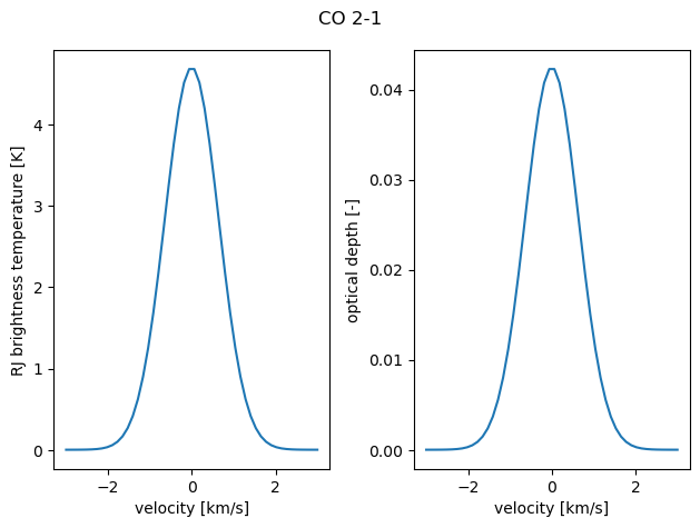
We can also get a spectrum of emission (i.e. emission as function of frequency) and the total optical depth at arbitrary frequencies. Note again that for a sphere, the optical depth calculated by pythonradex corresponds to the diameter of the sphere. It is often easiest to define a range of velocities and convert it to a frequency range. For the emission, we can request specific intensity (W/m2/Hz/sr), flux density (W/m2/Hz), Rayleigh-Jeans brightness temperature or Planck brightness temperature (both in K).

v = np.linspace(-2 * width_v, 2 * width_v, 50)  # m/s
# retrieve the rest frequency of CO 2-1
nu0 = source.emitting_molecule.nu0[1]  # Hz
nu = nu0 * (1 - v / constants.c)  # Hz
# total optical depth as function of nu, including dust
# and overlapping lines if present
tau = source.tau(nu=nu)
# total sprectrum (including dust and overlapping lines if present):
# we choose the output in the form of the Rayleigh-Jeans brightness temperature
# other options are "Planck" (Planck brightness temperture), "specific intensity" (W/m2/Hz/sr),
# and "flux density" (W/m2/Hz; for this option, a solid_angle needs to be provided)
spectrum = source.spectrum(output_type="Rayleigh-Jeans", nu=nu)

fig, axes = plt.subplots(ncols=2)
fig.suptitle("CO 2-1")
axes[0].plot(v / constants.kilo, spectrum)
axes[0].set_ylabel(r"RJ brightness temperature [K]")
axes[1].plot(v / constants.kilo, tau)
axes[1].set_ylabel("optical depth [-]")

for ax in axes:
    ax.set_xlabel("velocity [km/s]")
fig.tight_layout()

By the way, the same methods can also be used to get the emission or optical depth at a single frequency:

Delta_v = 0.5 * constants.kilo
offset_nu = nu0 + Delta_v / constants.c * nu0
offset_T_RJ = source.spectrum(nu=offset_nu, output_type="Rayleigh-Jeans")
print(
    f"Rayleigh-Jeans brightness temperature {Delta_v/constants.kilo:.2g} km/s offset from line center: {offset_T_RJ:.2g} K"
)
offset_tau = source.tau(nu=offset_nu)
print(
    f"optical depth {Delta_v/constants.kilo:.2g} km/s offset from line center: {offset_tau:.2g}"
)

Rayleigh-Jeans brightness temperature 0.5 km/s offset from line center: 3.5 K
optical depth 0.5 km/s offset from line center: 0.031

printing an overview of the results

An overview of the results can be printed to the console. For each transition, it lists the indices of the upper and lower level, the rest frequency, the excitation temperature, the fractional population of the lower and upper level, and the optical depth (for spheres, this is along the diameter) of the transition at the rest frequency

source.print_results()

  up   low      nu0 [GHz]    T_ex [K]      poplow         popup         tau_nu0
   1    0     115.271202     322.57      0.0371245        0.10948     0.00597971
   2    1     230.538000     174.39        0.10948        0.17125      0.0424729
   3    2     345.795990      99.95        0.17125        0.20307       0.148725
   4    3     461.040768      69.91        0.20307       0.190258       0.297295
   5    4     576.267931      55.49       0.190258       0.141269       0.390985
   6    5     691.473076      47.53       0.141269       0.083057       0.364103
   7    6     806.651806      43.71       0.083057      0.0395288       0.246477
   8    7     921.799700      43.18      0.0395288      0.0160823       0.126382
   9    8    1036.912393      44.74      0.0160823     0.00590993      0.0532576
  10    9    1151.985452      47.16     0.00590993     0.00202249      0.0199245
  11   10    1267.014486      49.99     0.00202249    0.000656319     0.00689005
  12   11    1381.995105      53.33    0.000656319    0.000205697     0.00224068
  13   12    1496.922909      56.93    0.000205697    6.28905e-05     0.00070135
  14   13    1611.793518      58.47    6.28905e-05    1.79922e-05    0.000217654
  15   14    1726.602506      59.68    1.79922e-05    4.79776e-06    6.31553e-05
  16   15    1841.345506      63.37    4.79776e-06    1.26639e-06    1.67294e-05
  17   16    1956.018139      64.25    1.26639e-06    3.11589e-07     4.4692e-06
  18   17    2070.615993      66.22    3.11589e-07    7.34479e-08    1.10241e-06
  19   18    2185.134680      68.90    7.34479e-08    1.68982e-08     2.5899e-07
  20   19    2299.569842      70.30    1.68982e-08    3.69662e-09     5.9773e-08
  21   20    2413.917113      71.23    3.69662e-09    7.62267e-10    1.31327e-08
  22   21    2528.172060      72.51    7.62267e-10    1.49675e-10    2.70884e-09
  23   22    2642.330346      74.04    1.49675e-10    2.81977e-11    5.31144e-10
  24   23    2756.387584      75.62    2.81977e-11    5.11227e-12    9.97404e-11
  25   24    2870.339407      76.59    5.11227e-12    8.80706e-13    1.80529e-11
  26   25    2984.181455      77.13    8.80706e-13     1.4293e-13    3.10642e-12
  27   26    3097.909361      77.95     1.4293e-13    2.20248e-14    5.02287e-13
  28   27    3211.518751      79.16    2.20248e-14    3.25705e-15     7.6954e-14
  29   28    3325.005283      80.79    3.25705e-15     4.6769e-16    1.12753e-14
  30   29    3438.364611      82.39     4.6769e-16    6.52602e-17    1.60358e-15
  31   30    3551.592361      82.24    6.52602e-17    8.48315e-18    2.22873e-16
  32   31    3664.684180      83.16    8.48315e-18     1.0559e-18    2.87172e-17
  33   32    3777.635728      83.57     1.0559e-18    1.24356e-19    3.54444e-18
  34   33    3890.442717      84.89    1.24356e-19     1.4197e-20    4.12249e-19
  35   34    4003.100788      85.52     1.4197e-20    1.54516e-21    4.65429e-20
  36   35    4115.605585      86.58    1.54516e-21    1.62299e-22    4.99803e-21
  37   36    4227.952774      87.38    1.62299e-22    1.63527e-23    5.18137e-22
  38   37    4340.138112      87.01    1.63527e-23    1.53224e-24    5.16228e-23
  39   38    4452.157122      88.35    1.53224e-24    1.40003e-25    4.75583e-24
  40   39    4564.005640      85.93    1.40003e-25    1.12204e-26    4.31115e-25

Change the source parameters

We can update the source parameters for another calculation using the update_parameters method. We can update a single parameter, or several parameters at the same time. We can update the column density, kinetic gas temperature, collider densities, external background, dust temperature and dust optical depth.

IMPORTANT: If you want to run pythonradex for a grid of parameters, do not initialise a new ``Source`` instance for each set of parameters! This is because setting up a new Source is computationally expensive, so the grid search will take much more time than needed. Instead, use the update_parameters method. Another notebook with an example grid search is available in the documentation.

For example, let’s change the kinetic temperature and solve again:

new_Tkin = 20
source.update_parameters(Tkin=new_Tkin)
source.solve_radiative_transfer()

for i in transition_indices:
    tau_nu0 = source.tau_nu0_individual_transitions[i]
    Tex = source.Tex[i]
    print(f"transition {i}: Tex = {Tex:.3g} K, tau_nu0 = {tau_nu0:.3g}")

transition 1: Tex = 19.2 K, tau_nu0 = 0.899
transition 2: Tex = 17.7 K, tau_nu0 = 1.05
transition 5: Tex = 14.1 K, tau_nu0 = 0.0439

The excitation temperatures are now much lower, as one might expected.