Comparing the outputs of pythonradex and RADEX

This notebook aims to provide a simple example of how to compare the excitation temperatures, optical depths and brightness temperatures calculated by pythonradex and RADEX.

Preparation

First, some preparation work is needed in order to use RADEX. Proceed as follows:

1. Download RADEX from the official RADEX page and install it according to the instructions. Make sure to choose “uniform sphere” as the geometry for the escape probability in radex.inc, as we will use that geometry in this example.

2. Download the file RADEX_wrapper.py from here and place it into the same folder as this notebook. In that file, modify the radex_path to point to your RADEX executable.

Single model

Run a single model with RADEX and pythonradex, and compare the outputs. Here we consider CO as an example.

from pythonradex import helpers, radiative_transfer
from scipy import constants
import os
import matplotlib.pyplot as plt
from matplotlib.colors import LogNorm
import numpy as np
import RADEX_wrapper

# define here the path to the folder that contains your LAMDA-formatted files
data_folder = "/home/gianni/science/LAMDA_database_files"

datafilename = "co.dat"
collider_densities = {"ortho-H2": 5e4 * constants.centi**-3}
# assume thermal ortho/para ratio:
collider_densities["para-H2"] = collider_densities["ortho-H2"] / 3
Tkin = 50
T_background = 2.73
N = 1e16 * constants.centi**-2
width_v = 2.3 * constants.kilo
# be careful with modifying the geometry. If you change the geometry for pythonradex,
# you also need to re-compile RADEX with the new geometry
# Also be careful when comparing to other geometries;
# - LVG sphere: RADEX and pythonradex use different escape probability (but you could use "LVG sphere RADEX")
# - static slab: not supported by RADEX
# - LVG slab: pythonradex only supports rectangular line profile
geometry = "static sphere"
# RADEX makes calculations using a rectangular profile, but it uses a correction factor to convert flux and optical
# depth to Gaussian, so choosing Gaussian is the appropriate choice for comparison with pythonradex
line_profile_type = "Gaussian"

source = radiative_transfer.Source(
    datafilepath=os.path.join(data_folder, datafilename),
    geometry=geometry,
    line_profile_type=line_profile_type,
    width_v=width_v,
)


def ext_background(nu):
    return helpers.B_nu(T=T_background, nu=nu)


source.update_parameters(
    ext_background=ext_background,
    N=N,
    Tkin=Tkin,
    collider_densities=collider_densities,
    T_dust=0,
    tau_dust=0,
)
source.solve_radiative_transfer()

# now run RADEX
radex_result = RADEX_wrapper.run(
    datafilename=datafilename,
    collider_densities=collider_densities,
    Tkin=Tkin,
    T_background=T_background,
    N=N,
    width_v=width_v,
    input_filepath="test.inp",
    output_filepath="test.out",
)

Let’s compare excitation temperatures, level populations and optical depths. Note that comparing intensities is not that straightforward, since RADEX and pythonradex compute intensities differently.

def plot_comparison(source, radex_result, yscale, max_E_up=np.inf):
    E_up = [
        trans.up.E / constants.k for trans in source.emitting_molecule.rad_transitions
    ]
    E_up = np.array(E_up)
    E_up_selection = E_up < max_E_up
    Tex = {"RADEX": radex_result["Tex"], "pythonradex": source.Tex}
    pop_up = {
        "RADEX": radex_result["pop_up"],
        "pythonradex": [
            source.level_pop[t.up.index]
            for t in source.emitting_molecule.rad_transitions
        ],
    }
    pop_low = {
        "RADEX": radex_result["pop_low"],
        "pythonradex": [
            source.level_pop[t.low.index]
            for t in source.emitting_molecule.rad_transitions
        ],
    }
    tau_nu0 = {
        "RADEX": radex_result["tau"],
        "pythonradex": source.tau_nu0_individual_transitions,
    }
    comparison_quantities = {
        "Tex": Tex,
        "tau_nu0": tau_nu0,
        "pop_up": pop_up,
        "pop_low": pop_low,
    }
    y_labels = {
        "Tex": "excitation temperature [K]",
        "pop_up": "upper level fractional population",
        "pop_low": "lower level fractional population",
        "tau_nu0": "optical depth",
    }
    fig, axes = plt.subplots(2, 2, figsize=(8, 8))
    marker = {"RADEX": "x", "pythonradex": "."}
    for ax, (quantity_name, quantity) in zip(
        axes.ravel(), comparison_quantities.items()
    ):
        for code, values in quantity.items():
            ax.plot(
                E_up[E_up_selection],
                np.array(values)[E_up_selection],
                marker[code],
                label=code,
            )
        if quantity_name == "Tex":
            ax.axhline(
                Tkin, linestyle="dashed", color="black", label="$T_\mathrm{kin}$"
            )
        ax.set_xlabel("upper level energy [K]")
        ax.set_ylabel(y_labels[quantity_name])
        ax.legend(loc="best")
        ax.set_yscale(yscale)
    fig.tight_layout()


plot_comparison(source=source, radex_result=radex_result, yscale="log")

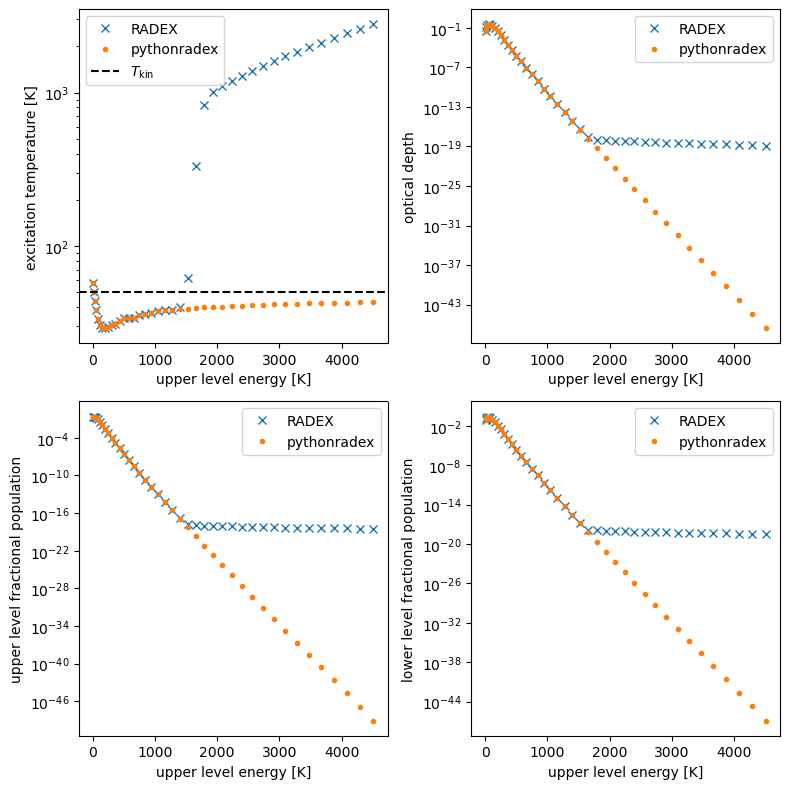
The agreement is good, except for excitation temperatures of transitions with very high upper level energy. Although the departure between RADEX and pythonradex looks dramatic for upper level energies exceeding ~1500 K, in practice it does not make a difference. Indeed, the corresponding levels are almost unpopulated (as expected, given that the kinetic temperature is much lower than the upper level energy), and thus the corresponding transitions are extremely weak (i.e. not observable).

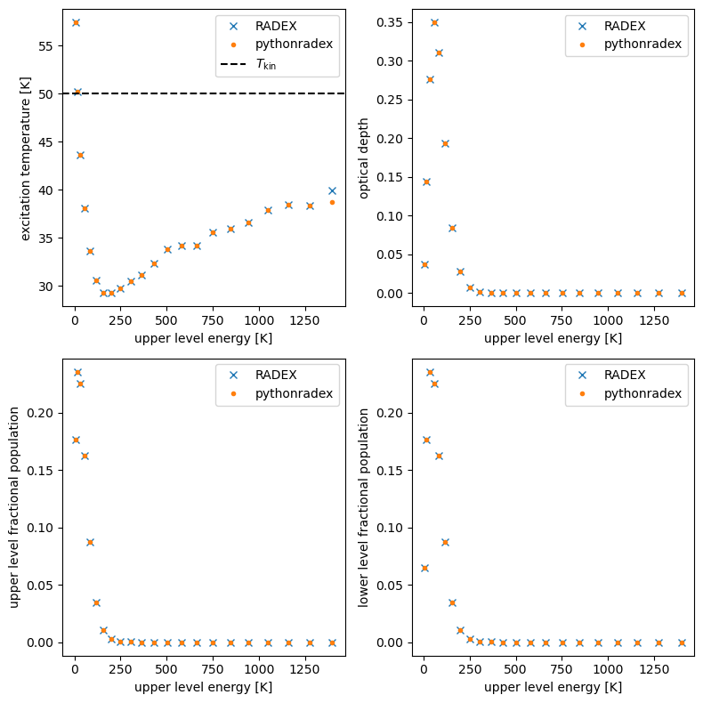
Let’s make the same plots, but in linear scale and restricting the upper level energies.

plot_comparison(
    source=source, radex_result=radex_result, yscale="linear", max_E_up=1500
)

Comparing intensities and brightness temperatures

Comparing intensities, respectively brightness temperatures, is not straightforward mainly for two reasons:

1. RADEX calculates background-subtracted intensities, while pythonradex just calculates the emission from the source and leaves and background subtraction to the user.

2. For spherical geometries, RADEX and pythonradex use different formulas to calculate the intensity (see the documentation for more details).

Thus, to compare intensities / brightness temperatures, some additional calculation is necessary. We transform the results from pythonradex such that they can be compared to RADEX.

nu0 = source.emitting_molecule.nu0  # all rest frequencies
tau_nu0 = source.tau_nu0_individual_transitions
# use the same formula as RADEX to calculate the specific intensity
specific_intensity_nu0 = helpers.B_nu(nu=nu0, T=source.Tex) * (1 - np.exp(-tau_nu0))
# now compute background subtraction
specific_intensity_nu0_bg_subtracted = (
    specific_intensity_nu0
    + ext_background(nu0) * np.exp(-tau_nu0)
    - ext_background(nu0)
)
# transform to Rayleigh-Jeans brightness temperature
TR_pythonradex_bg_subtracted = helpers.RJ_brightness_temperature(
    specific_intensity=specific_intensity_nu0_bg_subtracted, nu=nu0
)

# for comparison, also plot the RJ temperature computed by pythonradex
TR_pythonradex = source.emission_at_line_center(output_type="Rayleigh-Jeans")

fig, ax = plt.subplots()
ax.plot(TR_pythonradex, marker=".", label="pythonradex", linestyle="")
ax.plot(
    TR_pythonradex_bg_subtracted,
    marker="*",
    label="pythonradex using RADEX formulas",
    linestyle="",
)
ax.plot(radex_result["TR"], marker="x", label="RADEX", linestyle="")
ax.set_xlabel("transition index")
ax.set_ylabel("Rayleigh-Jeans brightness temperature [K]")
ax.legend(loc="best")

<matplotlib.legend.Legend at 0x7e53105b40e0>

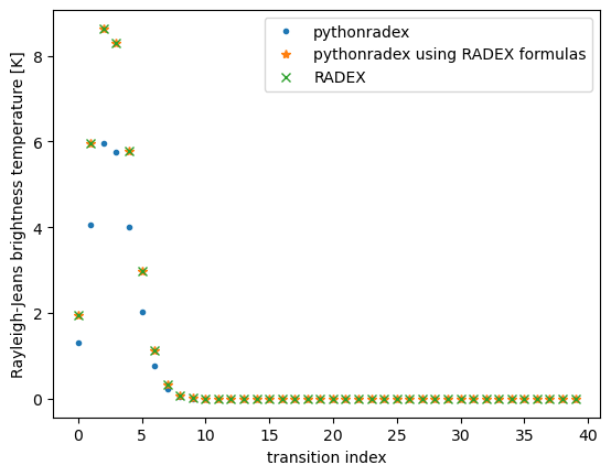
The agreement is excellent if the same formulas are used.

Negative excitation temperatures or optical depths

Both RADEX and pythonradex can produce unreliable results characterised by, for example, negative excitation temperatures. Let’s consider some extreme parameters: a column density of \(10^{18}\) cm\(^{-2}\) and a kinetic temperature of 1500 K.

N = 1e18 * constants.centi**-2
Tkin = 1500
source.update_parameters(N=N, Tkin=Tkin)
source.solve_radiative_transfer()

radex_result = RADEX_wrapper.run(
    datafilename=datafilename,
    collider_densities=collider_densities,
    Tkin=Tkin,
    T_background=T_background,
    N=N,
    width_v=width_v,
    input_filepath="test.inp",
    output_filepath="test.out",
)

plot_comparison(source=source, radex_result=radex_result, yscale="linear")

/home/gianni/science/projects/code/pythonradex_joss/pythonradex/src/pythonradex/radiative_transfer.py:417: UserWarning: negative optical depth!
  warnings.warn("negative optical depth!")

1-0: tau_nu0 = -0.0262
2-1: tau_nu0 = -0.0908
3-2: tau_nu0 = -0.202
4-3: tau_nu0 = -0.161

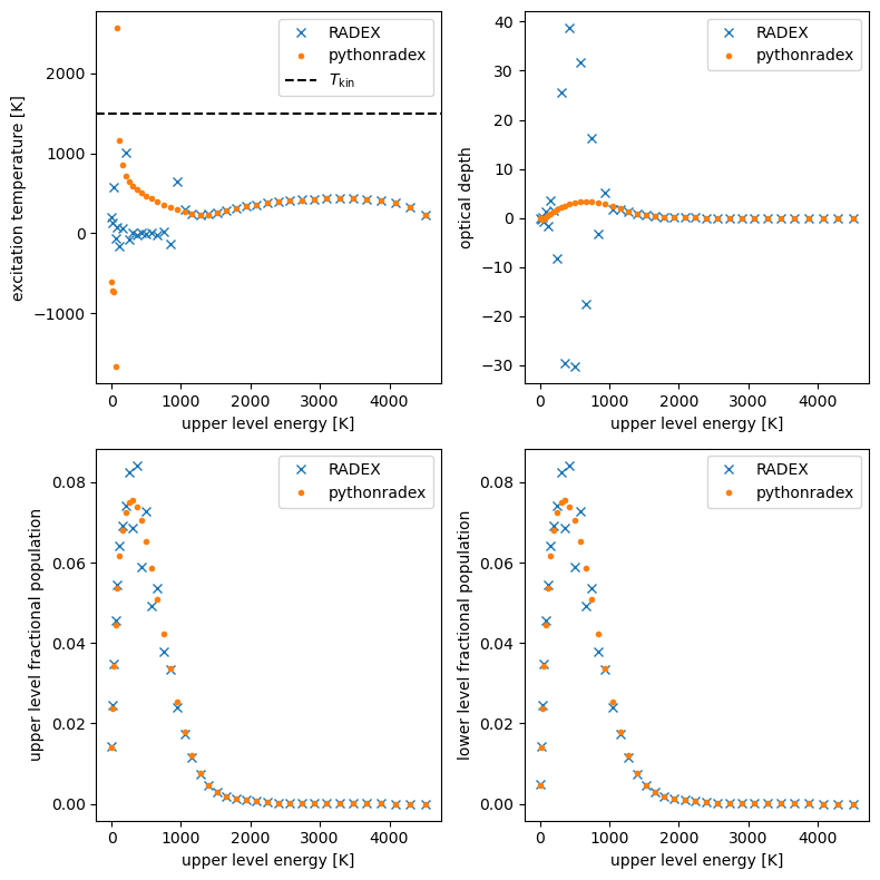
For this particular example, both RADEX and pythonradex predict negative excitation temperatures for transitions with low upper energy. Both codes also predict negative optical depth (RADEX for more transitions than pythonradex). These results are probably not reliable.

Model grid

Here we compare RADEX and pythonradex on a model grid. Let’s focus on CO 2-1. We calculate the excitation temperature and optical depth over a grid of H\(_2\) density and column density:

H2_grid = np.logspace(3, 7, 10) * constants.centi**-3
N_grid = np.logspace(13, 18, 15) * constants.centi**-2

# fix Tkin:
Tkin = 100
source.update_parameters(Tkin=Tkin)
trans_index = 1  # CO 2-1

Tex = {"RADEX": np.empty((H2_grid.size, N_grid.size))}
Tex["pythonradex"] = Tex["RADEX"].copy()
tau = {"RADEX": np.empty((H2_grid.size, N_grid.size))}
tau["pythonradex"] = tau["RADEX"].copy()

for i, nH2 in enumerate(H2_grid):
    # assume thermal ortho/para ratio
    collider_densities = {"ortho-H2": nH2 * 3 / 4, "para-H2": nH2 / 4}
    for j, N in enumerate(N_grid):
        source.update_parameters(N=N, collider_densities=collider_densities)
        source.solve_radiative_transfer()
        Tex["pythonradex"][i, j] = source.Tex[trans_index]
        tau["pythonradex"][i, j] = source.tau_nu0_individual_transitions[trans_index]
        radex_result = RADEX_wrapper.run(
            datafilename=datafilename,
            collider_densities=collider_densities,
            Tkin=Tkin,
            T_background=T_background,
            N=N,
            width_v=width_v,
            input_filepath="grid.inp",
            output_filepath="grid.out",
        )
        Tex["RADEX"][i, j] = radex_result["Tex"][trans_index]
        tau["RADEX"][i, j] = radex_result["tau"][trans_index]

Note: The following floating-point exceptions are signalling: IEEE_INVALID_FLAG
Note: The following floating-point exceptions are signalling: IEEE_INVALID_FLAG
Note: The following floating-point exceptions are signalling: IEEE_INVALID_FLAG

1-0: tau_nu0 = -0.000134
1-0: tau_nu0 = -0.000305
1-0: tau_nu0 = -0.000692

Note: The following floating-point exceptions are signalling: IEEE_INVALID_FLAG
Note: The following floating-point exceptions are signalling: IEEE_INVALID_FLAG
Note: The following floating-point exceptions are signalling: IEEE_INVALID_FLAG

1-0: tau_nu0 = -0.00157
1-0: tau_nu0 = -0.00355
1-0: tau_nu0 = -0.00796
1-0: tau_nu0 = -0.0175
1-0: tau_nu0 = -0.0371
1-0: tau_nu0 = -0.0725
1-0: tau_nu0 = -0.122
1-0: tau_nu0 = -0.152
1-0: tau_nu0 = -0.0653
1-0: tau_nu0 = -4.18e-05
1-0: tau_nu0 = -9.5e-05

Note: The following floating-point exceptions are signalling: IEEE_INVALID_FLAG
Note: The following floating-point exceptions are signalling: IEEE_INVALID_FLAG

1-0: tau_nu0 = -0.000216
1-0: tau_nu0 = -0.000491

Note: The following floating-point exceptions are signalling: IEEE_INVALID_FLAG
Note: The following floating-point exceptions are signalling: IEEE_INVALID_FLAG

1-0: tau_nu0 = -0.00112
1-0: tau_nu0 = -0.00253
1-0: tau_nu0 = -0.00569
1-0: tau_nu0 = -0.0126
1-0: tau_nu0 = -0.027
1-0: tau_nu0 = -0.0535
1-0: tau_nu0 = -0.0891
1-0: tau_nu0 = -0.0995

Note: The following floating-point exceptions are signalling: IEEE_INVALID_FLAG
Note: The following floating-point exceptions are signalling: IEEE_INVALID_FLAG
Note: The following floating-point exceptions are signalling: IEEE_INVALID_FLAG
Note: The following floating-point exceptions are signalling: IEEE_INVALID_FLAG
Note: The following floating-point exceptions are signalling: IEEE_INVALID_FLAG
Note: The following floating-point exceptions are signalling: IEEE_INVALID_FLAG
Note: The following floating-point exceptions are signalling: IEEE_INVALID_FLAG
Note: The following floating-point exceptions are signalling: IEEE_INVALID_FLAG
Note: The following floating-point exceptions are signalling: IEEE_INVALID_FLAG
Note: The following floating-point exceptions are signalling: IEEE_INVALID_FLAG
Note: The following floating-point exceptions are signalling: IEEE_INVALID_FLAG
Note: The following floating-point exceptions are signalling: IEEE_INVALID_FLAG
Note: The following floating-point exceptions are signalling: IEEE_INVALID_FLAG
Note: The following floating-point exceptions are signalling: IEEE_INVALID_FLAG
Note: The following floating-point exceptions are signalling: IEEE_INVALID_FLAG
Note: The following floating-point exceptions are signalling: IEEE_INVALID_FLAG
Note: The following floating-point exceptions are signalling: IEEE_INVALID_FLAG
Note: The following floating-point exceptions are signalling: IEEE_INVALID_FLAG
Note: The following floating-point exceptions are signalling: IEEE_INVALID_FLAG
Note: The following floating-point exceptions are signalling: IEEE_INVALID_FLAG
Note: The following floating-point exceptions are signalling: IEEE_INVALID_FLAG
Note: The following floating-point exceptions are signalling: IEEE_INVALID_FLAG
Note: The following floating-point exceptions are signalling: IEEE_INVALID_FLAG
Note: The following floating-point exceptions are signalling: IEEE_INVALID_FLAG
Note: The following floating-point exceptions are signalling: IEEE_INVALID_FLAG
Note: The following floating-point exceptions are signalling: IEEE_INVALID_FLAG
Note: The following floating-point exceptions are signalling: IEEE_INVALID_FLAG
Note: The following floating-point exceptions are signalling: IEEE_INVALID_FLAG
Note: The following floating-point exceptions are signalling: IEEE_INVALID_FLAG
Note: The following floating-point exceptions are signalling: IEEE_INVALID_FLAG
Note: The following floating-point exceptions are signalling: IEEE_INVALID_FLAG
Note: The following floating-point exceptions are signalling: IEEE_INVALID_FLAG
Note: The following floating-point exceptions are signalling: IEEE_INVALID_FLAG
Note: The following floating-point exceptions are signalling: IEEE_INVALID_FLAG
Note: The following floating-point exceptions are signalling: IEEE_INVALID_FLAG
Note: The following floating-point exceptions are signalling: IEEE_INVALID_FLAG
Note: The following floating-point exceptions are signalling: IEEE_INVALID_FLAG
Note: The following floating-point exceptions are signalling: IEEE_INVALID_FLAG

You might see Fortran warnings raised by RADEX (“Note: The following floating-point exceptions are signalling: IEEE_INVALID_FLAG”), but you don’t need to worry about them here. We first inspect the excitation temperature for each code:

H2_GRID, N_GRID = np.meshgrid(H2_grid, N_grid, indexing="ij")
fig, axes = plt.subplots(ncols=2)
for ax, (code, Tex_values) in zip(axes.ravel(), Tex.items()):
    im = ax.pcolormesh(
        H2_GRID / constants.centi**-3,
        N_GRID / constants.centi**-2,
        Tex_values,
        norm=LogNorm(vmin=Tex_values.min(), vmax=Tex_values.max()),
    )
    cbar = fig.colorbar(im, ax=ax, orientation="horizontal", location="top")
    cbar.ax.xaxis.set_label_position("top")
    cbar.ax.xaxis.set_ticks_position("top")
    cbar.set_label(f"Tex [K] ({code})", labelpad=10)
    ax.set_xscale("log")
    ax.set_yscale("log")
    ax.set_xlabel("H$_2$ density [cm$^{-3}$]")
    ax.set_ylabel("column density [cm$^{-2}$]")
fig.tight_layout()

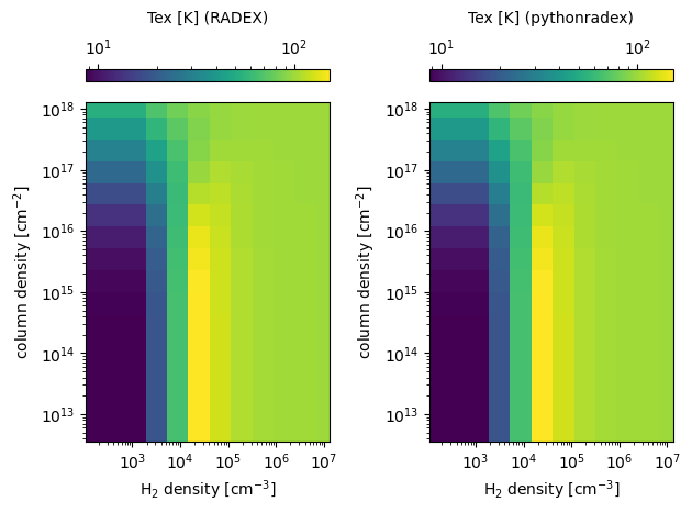
Looks like both codes produces similar excitation temperatures. Also, both codes correctly reproduce the LTE limit (high H\(_2\) density) where the excitation temperature should equal the kinetic temperature.

Let’s also look at the ratio to check how large the difference between the two codes is:

def plot_ratio(ratio, label):
    fig, ax = plt.subplots()
    min_ratio, max_ratio = np.min(ratio), np.max(ratio)
    assert 0 < min_ratio <= 1
    assert 1 <= max_ratio
    # set limits of the colorbar such that 1 is in the center:
    max_deviation_from_1 = np.max(np.abs(ratio - 1))
    vmin = 1 - max_deviation_from_1
    vmax = 1 + max_deviation_from_1
    im = ax.pcolormesh(
        H2_GRID / constants.centi**-3,
        N_GRID / constants.centi**-2,
        ratio,
        cmap="seismic",
        vmin=vmin,
        vmax=vmax,
    )
    cbar = fig.colorbar(im, ax=ax, orientation="horizontal", location="top")
    cbar.ax.xaxis.set_label_position("top")
    cbar.ax.xaxis.set_ticks_position("top")
    cbar.set_label(label, labelpad=10)
    ax.set_xscale("log")
    ax.set_yscale("log")
    ax.set_xlabel("H$_2$ density [cm$^{-3}$]")
    ax.set_ylabel("column density [cm$^{-2}$]")
    fig.tight_layout()


plot_ratio(
    ratio=Tex["pythonradex"] / Tex["RADEX"],
    label="$T_\mathrm{ex}^\mathrm{pythonradex}/T_\mathrm{ex}^{RADEX}$",
)

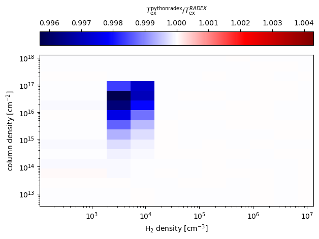
The agreement is extremely good, wich deviations less than 1%. Similarly, let us compare optical depths:

plot_ratio(
    ratio=tau["pythonradex"] / tau["RADEX"],
    label=r"$\tau^\mathrm{pythonradex}/\tau^{RADEX}$",
)

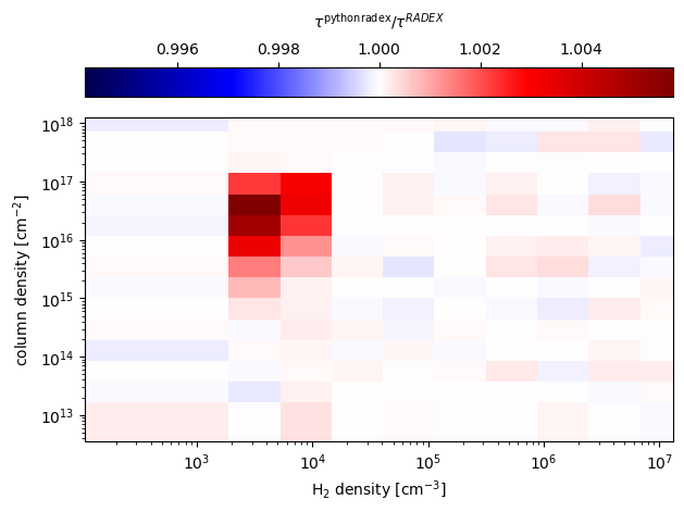
Again, the agreement is very good, with deviations less than a 1%.