Line core saturation by high optical depth

Let’s check how optical depth affects the spectrum by saturating the line core. We need to consider a Gaussian line profile to see this effect. Let’s initialise the source:

from pythonradex import radiative_transfer, helpers
from scipy import constants
import numpy as np
import matplotlib.pyplot as plt

width_v = 1 * constants.kilo
source = radiative_transfer.Source(
    datafilepath="./co.dat",
    geometry="static slab",
    line_profile_type="Gaussian",
    width_v=1 * constants.kilo,
)
# we put a high column density to force high optical depth. We do not
# consider dust effects.
collider_densities = {
    "para-H2": 1e3 / constants.centi**3,
    "ortho-H2": 3e3 / constants.centi * 3,
}
source.update_parameters(
    N=1e18 / constants.centi**2,
    Tkin=50,
    collider_densities=collider_densities,
    ext_background=helpers.generate_CMB_background(),
    T_dust=0,
    tau_dust=0,
)
source.solve_radiative_transfer()
index_21 = 1  # the 2-1 transition is listed 2nd in the LAMDA file,
# so its index is 1
print(f"tau_nu0 of CO 2-1: {source.tau_nu0_individual_transitions[index_21]:.3g}")

tau_nu0 of CO 2-1: 34.8

The line is very optically thick. Let’s take a look at the spectrum of CO 2-1

v = np.linspace(-2 * width_v, 2 * width_v, 50)
nu0_21 = source.emitting_molecule.nu0[index_21]  # rest frequency of CO 2-1
nu = nu0_21 * (1 - v / constants.c)

spectrum = source.spectrum(output_type="specific intensity", nu=nu)
tau = source.tau(nu=nu)

fig, axes = plt.subplots(ncols=2)
fig.suptitle("CO 2-1")
axes[0].plot(v / constants.kilo, spectrum)
axes[0].set_title("spectrum")
axes[0].set_ylabel(r"specific intensity [W/m$^2$/Hz/sr]")
axes[0].yaxis.set_major_formatter(plt.ScalarFormatter(useMathText=True))
axes[1].plot(v / constants.kilo, tau)
axes[1].set_title("optical depth")
axes[1].set_ylabel(r"tau [-]")
for ax in axes:
    ax.set_xlabel("velocity [km/s]")
fig.tight_layout()

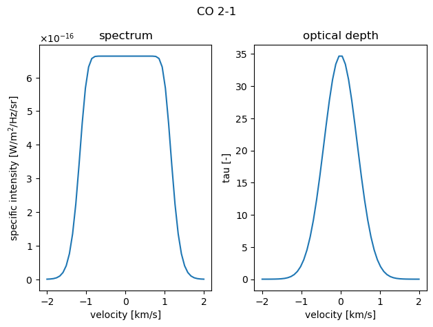
We can clearly see the saturated core of the spectrum.